Now, here's the rub. The slicers still work, but they don't filter the 'YearFilter' field, they actually filter the Year field in the PivotTable. Despite the fact that the data is the same, it won't quite work. To fix this, delete the Slicer, and re-create it against the 'YearFilter' field instead of the 'Year' field. Nov 01, 2017  Slicers on charts are not supported in Excel for Mac. It has nothing to do with updates. The Excel product manager makes this distinction in the 'wish we had' forum here.

When you create a new Excel pivot table, you’ll notice that Excel 2019 automatically adds drop-down buttons to the Report Filter field, as well as the labels for the column and row fields. These drop-down buttons, known officially as filter buttons in Excel, enable you to filter all but certain entries in any of these fields, and in the case of the column and row fields, to sort their entries in the table.

If you’ve added more than one column or row field to your pivot table, Excel adds collapse buttons (-) that you can use to temporarily hide subtotal values for a particular secondary field. After clicking a collapse button in the table, it immediately becomes an expand button (+) that you can click to redisplay the subtotals for that one secondary field.

Filtering pivot tables in Excel 2019

Perhaps the most important filter buttons in an Excel pivot table are the ones added to the field(s) designated as the pivot table FILTERS. By selecting a particular option on the drop-down lists attached to one of these filter buttons, only the summary data for that subset you select displays in the pivot table.

For example, in the sample Excel pivot table that uses the Gender field from the Employee Data list as the Report Filter field, you can display the sum of just the men’s or women’s salaries by department and location in the body of the pivot table doing either of the following:

• Click the Gender field’s filter button and then click M on the drop-down list before you click OK to see only the totals of the men’s salaries by department.
• Click the Gender field’s filter button and then click F on the drop-down list before you click OK to see only the totals of the women’s salaries by department.

When you later want to redisplay the summary of the salaries for all the employees, you then reselect the (All) option on the Gender field’s drop-down filter list before you click OK.

When you filter the Gender Report Filter field in this manner, Excel then displays M or F in the Gender Report Filter field instead of the default (All). The program also replaces the standard drop-down button with a cone-shaped filter icon, indicating that the field is filtered and showing only some of the values in the data source.

Filtering column and row fields

The filter buttons on the column and row fields attached to their labels enable you to filter out entries for particular groups and, in some cases, individual entries in the data source. To filter the summary data in the columns or rows of a pivot table, click the column or row field’s filter button and start by clicking the check box for the (Select All) option at the top of the drop-down list to clear this box of its check mark. Then, click the check boxes for all the groups or individual entries whose summed values you still want displayed in the pivot table to put back check marks in each of their check boxes. Then click OK.

As with filtering a Report Filter field, Excel replaces the standard drop-down button for that column or row field with a cone-shaped filter icon, indicating that the field is filtered and displaying only some of its summary values in the pivot table. To redisplay all the values for a filtered column or row field, you need to click its filter button and then click (Select All) at the top of its drop-down list. Then click OK.

This image shows the sample pivot table after filtering its Gender Report Filter field to women (by selecting F in the Gender drop-down list) and its Dept Column field to Accounting, Administration, and Human Resources.

In addition to filtering out individual entries in an Excel pivot table, you can also use the options on the Label Filters and Value Filters continuation menus to filter groups of entries that don’t meet certain criteria, such as company locations that don’t start with a particular letter or salaries between $45,000 and $65,000.

Filtering in Excel with slicers

Slicers in Excel 2019 make it a snap to filter the contents of your pivot table on more than one field. (They even allow you to connect with fields of other pivot tables that you’ve created in the Excel workbook.)

To add slicers to your Excel pivot table, you follow just two steps:

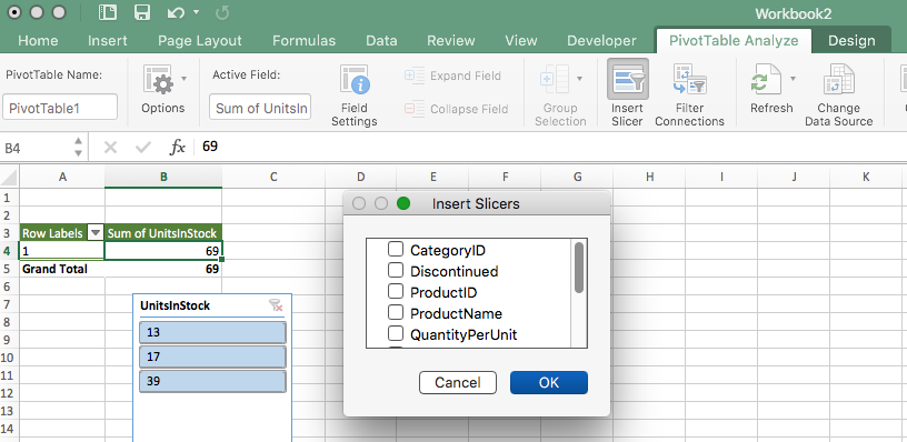
1. Click one of the cells in your pivot table to select it and then click the Insert Slicer button located in the Filter group of the Analyze tab under the PivotTable Tools contextual tab.
   Excel opens the Insert Slicers dialog box with a list of all the fields in the active pivot table.
2. Select the check boxes for all the fields that you want to use in filtering the pivot table and for which you want slicers created and then click OK.
   Excel then adds slicers (as graphic objects) for each pivot table field you select and automatically closes the PivotTable Fields task pane if it’s open at the time.

After you create slicers for the Excel pivot table, you can use them to filter its data simply by selecting the items you want displayed in each slicer. You select items in a slicer by clicking them just as you do cells in a worksheet — hold down Ctrl as you click nonconsecutive items and Shift to select a series of sequential items. For additional help, check out these other entry shortcuts.

The image below shows you the sample pivot table after using slicers created for the Gender, Dept, and Location fields to filter the data so that only salaries for the men in the Human Resources and Administration departments in the Boston, Chicago, and San Francisco offices display.

Because slicers are Excel graphic objects (albeit some pretty fancy ones), you can move, resize, and delete them just as you would any other Excel graphic. To remove a slicer from your pivot table, click it to select it and then press the Delete key.

Filtering with timelines in Excel

Excel 2019 offers another fast and easy way to filter your data with its timeline feature. You can think of timelines as slicers designed specifically for date fields that enable you to filter data out of your pivot table that doesn’t fall within a particular period, thereby allowing you to see timing of trends in your data.

To create a timeline for your Excel pivot table, select a cell in your pivot table and then click the Insert Timeline button in the Filter group on the Analyze contextual tab under the PivotTable Tools tab on the Ribbon. Excel then displays an Insert Timelines dialog box displaying a list of pivot table fields that you can use in creating the new timeline. After selecting the check box for the date field you want to use in this dialog box, click OK.

This image shows you a timeline created for the sample Employee Data list by selecting its Date Hired field in the Insert Timelines dialog box. As you can see, Excel created a floating Date Hired timeline with the years and months demarcated and a bar that indicates the time period selected. By default, the timeline uses months as its units, but you can change this to years, quarters, or even days by clicking the MONTHS drop-down button and selecting the desired time unit.

Then the timeline is literally used to select the period for which you want the Excel pivot table data displayed. In the image above, Excel pivot table has been filtered so that it shows the salaries by department and location for only employees hired in the year 2000. You can do this simply by dragging the timeline bar in the Date Hired timeline graphic so that it begins at Jan, 2000 and extends just up to and including Dec, 2000. And to filter the pivot table salary data for other hiring periods, simply modify the start and stop times by dragging the timeline bar in the Date Hired timeline.

Sorting pivot tables in Excel 2019

You can instantly reorder the summary values in a pivot table by sorting the table on one or more of its column or row fields. To re-sort a pivot table, click the filter button for the column or row field you want to use in the sorting and then click the Sort A to Z option or the Sort Z to A option at the top of the field’s drop-down list.

Click the Sort A to Z option when you want the table re-ordered by sorting the labels in the selected field alphabetically or, in the case of values, from the smallest to largest value or, in the case of dates, from the oldest to newest date. Click the Sort Z to A option when you want the table re-ordered by sorting the labels in reverse alphabetical order, values from the highest to smallest, and dates from the newest to oldest.

-->

Notice

Excel Viewer has been retired

Important

The Microsoft Excel Viewer was retired in April, 2018. It is no longer available for download or receive security updates. To continue viewing Excel files for free, we recommend installing the Excel mobile app or storing documents in OneDrive or Dropbox, where Excel Online opens them in your browser. For the Excel mobile app, visit the store for your device:

Summary

The Microsoft Excel Viewer is a small, freely redistributable program that lets you view and print Microsoft Excel spreadsheets if you don’t have Excel installed. In addition, the Excel Viewer can open workbooks that were created in Microsoft Excel for the Macintosh.

The Excel Viewer can open the latest version of Excel workbooks, but it will not display newer features.

More Information

The Microsoft Excel Viewer is the latest version of the viewer. It can read the file formats of all versions of Excel, and it replaces the Microsoft Excel Viewer 2003.

Other options for free viewing of Excel workbooks

• Excel Online Excel Online is available through OneDrive or deployed as part of Microsoft SharePoint. Excel Online can view, edit and print Excel workbooks. For more information about Excel Online, see the Office Online overview.
• Office 365 Trial Downloading the trial will give you access to the full capabilities of Microsoft Office 2013. For more information, see Office 365 Home.
• Office Mobile applications Download the trial for mobile applications available on iPhone, Android phone, or Windows Phone. For more information, see Office on mobile devices.

Note

The Excel Viewer is available only as a 32-bit application. A 64-bit version of the Excel Viewer does not exist. The 32-bit version of the Excel Viewer can be used on 64-bit versions of Windows.

The file name of the Excel Viewer is xlview.exe. The default folder location for the Excel Viewer on a 32-bit operating system isc:Program FilesMicrosoft OfficeOffice12. The default folder location for the Excel Viewer on a 64-bit operating system is c:Program Files (x86)Microsoft OfficeOffice12.

Note

If you already have a full version of Microsoft Excel installed on your computer, do not install Microsoft Excel Viewer in the same directory. Doing this causes file conflicts.

File formats supported

The Excel file formats supported are .xlsx, .xlsm, .xlsb, .xltx, .xltm, .xls, .xlt, .xlm, and .xlw. Macro-enabled files can be opened (.xlsm, .xltm, and .xlm), but the macros do not run.

Known issues with newer versions of Excel workbooks and the Excel Viewer

Even though the Excel Viewer can read the latest Excel workbooks, the following new features are not visible or are displayed differently in the Excel Viewer.

• Sparklines are not shown in the Excel Viewer. The cells where they are located are blank.

• PivotTables and PivotCharts are flattened. The data or chart will appear, but modifications cannot be made.

• Macros do not run in the Excel Viewer.

• Slicers do not display data in the Excel Viewer. Instead, a box is displayed in the location of the slicer and it contains the following text: 'This shape represents a slicer. Slicers are supported in Excel 2010 or later. If the shape was modified in an earlier version of Excel, or if the workbook was saved in Excel 2003 or earlier, the slicer cannot be used.'

If you have to view or use these features, use Excel Online.