Slicers In Excel For Mac

суббота 01 февраля22.08.2017admin

Slicers were introduced in Excel 2010, and they make it easy to change multiple pivot tables with a single click

Video: Add Slicers to Filter Pivot Table Data

The slicer is connected to both pivot tables. Remove all fields from the areas of the new pivot table. Add the slicer field to the Filters area of the new pivot table. Move the slicer on top of the cell that contains the filter drop-down button in the Filters area of the new pivot table. Excel Slicer Formatting. The trick is to create your own custom Slicer style. Step 1: Select a Slicer to reveal the contextual Slicer Tools; Options tab. Step 2: In the Slicer Styles gallery choose a style that’s close to what you want. Trust me, this will save you time.

In this video you can see the steps for adding a slicer to a pivot table in Excel 2010, and then using slicers to filter the data. The written instructions are below the video.

Add Slicers to Filter Pivot Table Data

Introduced in Excel 2010, Slicers are a powerful new way to filter pivot table data.

It's easy to add a Slicer:

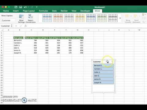
Select a cell in the pivot table
On the Ribbon's Insert tab, click Slicer.
In the list of pivot table fields, add check marks for the slicer(s) you want to create
Move and resize the slicers, if necessary, so they fit on the empty areas of the worksheet
Click on an item in a Slicer, to filter the pivot table. Other Slicers will show related items at the top.

Video: Filter Multiple Pivot Tables With One Slicer

In this video, you'll see the steps for connecting multiple pivot tables to a slicer, so they can all be filtered with a single click.

Video: Change All Pivot Charts With One Filter

This video shows how you can use a single Report Filter, connected to a slicer, to update multiple pivot charts. The slicers are stored on a different worksheet, so they don't take up room on your Excel dashboard sheet.

Watch this video to see how to set up the pivot tables and the pivot charts, and connect them to the slicer.

Video: Problem With Drill to Detail and Slicers

Slicers, combined with a pivot table's Drill to Detail feature, can produce unexpected results. See the problem in this video.

Video: Problems With Adding Slicers

Update older Excel files, if you want to use Slicers with the pivot tables in those files. Occasionally, there is a problem updating a pivot table, so you can try to repair it, by following the steps in this video.

Written instructions are below the video.

Problems With Adding Slicers

Usually it's easy to add a Slicer to a pivot table, but for files that were created in older versions of Excel, you might need to update the file before adding Slicers.

To use Slicers in a pivot table created in Excel 2003, follow these steps to update the file to a newer format:

Open the file (xls format) in Excel 2010. The file name will appear in the title bar of the Excel window, and it will show [Compatibility Mode] after the file name.
Click the File tab on the Ribbon, and click Save As
From the Save As Type drop down list, select Excel Workbook (xlsx), or select macro-enabled workbook (xlsm) if the file contains macros.
Enter a name and select a folder, and click the Save button.
The file is updated to the new format, and you can see that extension in the file name in the title bar.

After you update the file, the title bar will still show [Compatibility Mode] after the file name. Follow these steps to complete the update:

Close the updated file, and then re-open it.
The [Compatibility Mode] after the file name will have disappeared, and you should be able to select a pivot table cell, and add a Slicer.

Update Files Won't Allow Slicers

After following these steps, most files will allow you to add Slicers to the pivot tables. However, the occasional file might not show an enabled Slicer button, even after updating.

If you encounter that problem, there is probably some corruption in the old pivot table,

You can build a new pivot table from the source data, and delete the old one.
Or, you can try to repair the pivot table, by following the steps below.

To try to repair the pivot table:

Open the file in Excel 2010, and click the File tab on the Ribbon.
Click Save As, and save the file in Excel 97-2003 format (xls). Click Continue if a Compatibility Checker appears, listing the features that might be affected.
Close the file, and re-open it.
If an unreadable content message appears, click Yes, to open the file.
If a Repair message appears, click Close, after reading the repairs information.
The title bar will show the .xls file format, and [Repaired] and [Compatibiltiy Mode]

The final step is to save the file back into the newer format.

Click Save As, and save the file in Excel 2010 format (xlsx or xlsm).
Close the file, and re-open it. The title bar should show the file name, without [Repaired] or [Compatibiltiy Mode].

Then, select a cell in the pivot table, and if the repair was successful, you will be able to insert a Slicer.

Download the Sample File

If you need sample data to test with these pivot table Slicer videos, click here to download a zipped sample file with Region Sales data. It also has a pivot table with two Slicers set up. The zipped file is in xlsx format, and does not contain macros.

Filtering pivot tables in Excel 2019

Perhaps the most important filter buttons in an Excel pivot table are the ones added to the field(s) designated as the pivot table FILTERS. By selecting a particular option on the drop-down lists attached to one of these filter buttons, only the summary data for that subset you select displays in the pivot table.

For example, in the sample Excel pivot table that uses the Gender field from the Employee Data list as the Report Filter field, you can display the sum of just the men’s or women’s salaries by department and location in the body of the pivot table doing either of the following:

Click the Gender field’s filter button and then click M on the drop-down list before you click OK to see only the totals of the men’s salaries by department.
Click the Gender field’s filter button and then click F on the drop-down list before you click OK to see only the totals of the women’s salaries by department.

When you later want to redisplay the summary of the salaries for all the employees, you then reselect the (All) option on the Gender field’s drop-down filter list before you click OK.

When you filter the Gender Report Filter field in this manner, Excel then displays M or F in the Gender Report Filter field instead of the default (All). The program also replaces the standard drop-down button with a cone-shaped filter icon, indicating that the field is filtered and showing only some of the values in the data source.

Filtering column and row fields

The filter buttons on the column and row fields attached to their labels enable you to filter out entries for particular groups and, in some cases, individual entries in the data source. To filter the summary data in the columns or rows of a pivot table, click the column or row field’s filter button and start by clicking the check box for the (Select All) option at the top of the drop-down list to clear this box of its check mark. Then, click the check boxes for all the groups or individual entries whose summed values you still want displayed in the pivot table to put back check marks in each of their check boxes. Then click OK.

As with filtering a Report Filter field, Excel replaces the standard drop-down button for that column or row field with a cone-shaped filter icon, indicating that the field is filtered and displaying only some of its summary values in the pivot table. To redisplay all the values for a filtered column or row field, you need to click its filter button and then click (Select All) at the top of its drop-down list. Then click OK.

This image shows the sample pivot table after filtering its Gender Report Filter field to women (by selecting F in the Gender drop-down list) and its Dept Column field to Accounting, Administration, and Human Resources.

In addition to filtering out individual entries in an Excel pivot table, you can also use the options on the Label Filters and Value Filters continuation menus to filter groups of entries that don’t meet certain criteria, such as company locations that don’t start with a particular letter or salaries between $45,000 and $65,000.

Filtering in Excel with slicers

Slicers in Excel 2019 make it a snap to filter the contents of your pivot table on more than one field. (They even allow you to connect with fields of other pivot tables that you’ve created in the Excel workbook.)

To add slicers to your Excel pivot table, you follow just two steps:

Click one of the cells in your pivot table to select it and then click the Insert Slicer button located in the Filter group of the Analyze tab under the PivotTable Tools contextual tab.
Excel opens the Insert Slicers dialog box with a list of all the fields in the active pivot table.
Select the check boxes for all the fields that you want to use in filtering the pivot table and for which you want slicers created and then click OK.
Excel then adds slicers (as graphic objects) for each pivot table field you select and automatically closes the PivotTable Fields task pane if it’s open at the time.

After you create slicers for the Excel pivot table, you can use them to filter its data simply by selecting the items you want displayed in each slicer. You select items in a slicer by clicking them just as you do cells in a worksheet — hold down Ctrl as you click nonconsecutive items and Shift to select a series of sequential items. For additional help, check out these other entry shortcuts.

The image below shows you the sample pivot table after using slicers created for the Gender, Dept, and Location fields to filter the data so that only salaries for the men in the Human Resources and Administration departments in the Boston, Chicago, and San Francisco offices display.

Because slicers are Excel graphic objects (albeit some pretty fancy ones), you can move, resize, and delete them just as you would any other Excel graphic. To remove a slicer from your pivot table, click it to select it and then press the Delete key.

Filtering with timelines in Excel

Excel 2019 offers another fast and easy way to filter your data with its timeline feature. You can think of timelines as slicers designed specifically for date fields that enable you to filter data out of your pivot table that doesn’t fall within a particular period, thereby allowing you to see timing of trends in your data.

To create a timeline for your Excel pivot table, select a cell in your pivot table and then click the Insert Timeline button in the Filter group on the Analyze contextual tab under the PivotTable Tools tab on the Ribbon. Excel then displays an Insert Timelines dialog box displaying a list of pivot table fields that you can use in creating the new timeline. After selecting the check box for the date field you want to use in this dialog box, click OK.

This image shows you a timeline created for the sample Employee Data list by selecting its Date Hired field in the Insert Timelines dialog box. As you can see, Excel created a floating Date Hired timeline with the years and months demarcated and a bar that indicates the time period selected. By default, the timeline uses months as its units, but you can change this to years, quarters, or even days by clicking the MONTHS drop-down button and selecting the desired time unit.

Then the timeline is literally used to select the period for which you want the Excel pivot table data displayed. In the image above, Excel pivot table has been filtered so that it shows the salaries by department and location for only employees hired in the year 2000. You can do this simply by dragging the timeline bar in the Date Hired timeline graphic so that it begins at Jan, 2000 and extends just up to and including Dec, 2000. And to filter the pivot table salary data for other hiring periods, simply modify the start and stop times by dragging the timeline bar in the Date Hired timeline.

Sorting pivot tables in Excel 2019

You can instantly reorder the summary values in a pivot table by sorting the table on one or more of its column or row fields. To re-sort a pivot table, click the filter button for the column or row field you want to use in the sorting and then click the Sort A to Z option or the Sort Z to A option at the top of the field’s drop-down list.

Click the Sort A to Z option when you want the table re-ordered by sorting the labels in the selected field alphabetically or, in the case of values, from the smallest to largest value or, in the case of dates, from the oldest to newest date. Click the Sort Z to A option when you want the table re-ordered by sorting the labels in reverse alphabetical order, values from the highest to smallest, and dates from the newest to oldest.